Description

In This project, I performed a landmark-based Extended Kalman Filtered (EKF) SLAM on Turtlebot3. I used unsupervised learning with known and unknown data association for simultaneous localization and mapping of the environment.
I implemented the project from scratch using ROS in C++.

Take a look at the project on my GitHub page or read the package documentation.

Demo of the EKF-SLAM algorithm in action

Overview

Packages

The project contains 6 core ROS packages:

1. nuturtle_descritopn - A package that adapts the URDF model of turtlebot3_burger, a differential drive robot, for rviz visualization.
2. rigid2d - A 2D Lie Group library used for transformation, vectors and twist operations in 2D for differential drive robots.
3. trect - A package for waypoints following feedback control.
4. nuturtle_robot - A package for Turtlebot3 hardware interface, including setting motor control and getting Lidar readings.
5. nuturtlesim - A package that simulates the kinematics of the diff-drive turtlebot.
6. nuslam - A package contains the implementations of the feature detection algorithm and the feature-based Kalman Filter SLAM.

Main Algorithms

The SLAM pipeline can be describe using the following diagram:

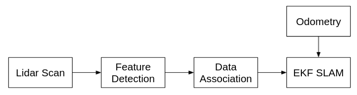
Project block diagram

Where the system gets measurements from the Lidar, performs feature detection using circle regression to find the landmarks location, Associating the measured data to the known landmarks, and update EKF SLAM using the associated landmarks and odometry calculations.

Here are some explanations about the mentioned algorithms:

Odometry

The library rigid2d performs two-dimensional rigid body transformations, and the library diff_drive performs the kinematics of a differential drive robot. The latter's main purpose is to convert wheel velocity to body twist and vice versa, and derive the odometry.

Twist to wheel velocity

According to$^{[2]}$, we can write the twist of each wheel as: $$ V_i = A_{ib}\cdot V_b $$ Where $$ V = \begin{bmatrix} \dot\theta \\ V_x \\ V_y \end{bmatrix} $$ and $$ A_{ib} = \begin{bmatrix} 1 && 0 && 0 \\ Base && 1 && 0 \\ 0 && 0 && 1 \end{bmatrix} $$ $ Base = D $ for wheel 1, and $ Base = -D $ for wheel 2.

The following sketch describes the robot's frames and dimensions:

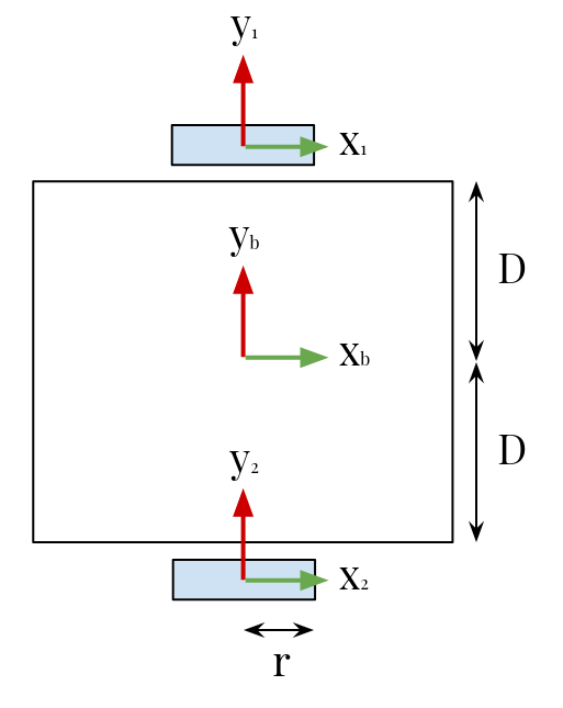
Differential drive robot description, where $D$ is the wheel base distance ans $r$ is the wheel radius

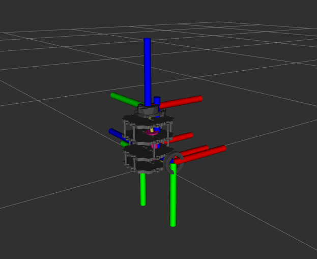
Visualizing the turtlebot's frames in Rviz

In conventional wheel we assume no slipping and no sliding ($V_y = 0$). Therefore: $$ \begin{bmatrix} \dot\theta \\ V_{xi} \\ V_{yi} \end{bmatrix} = \begin{bmatrix} 1 && 0 && 0 \\ Base && 1 && 0 \\ 0 && 0 && 1 \end{bmatrix} \begin{bmatrix} \dot\theta \\ r\dot\phi_i \\ 0 \end{bmatrix} $$ Where $ \dot\phi_i $ is the rotational velocity of wheel $i$ and $r$ is the wheel radius.

Now, by extracting $ \dot\phi_i $, we can find the connection between wheel velocity and twist: $$ \underbrace{ \begin{bmatrix} \dot\phi_1 \\ \dot\phi_2 \end{bmatrix}}_u = \frac{1}{r} \underbrace{ \begin{bmatrix} -D && 1 && 0 \\ +D && 1 && 0 \end{bmatrix}}_H \underbrace{ \begin{bmatrix} \dot\theta \\ V_x \\ V_y \end{bmatrix}}_{V_b} $$

Wheel velocity to twist

From$^{[2]}$, we can find the control to twist relationship by solving $ u = HV_b $ for $ V_b $ as: $$ V_b = H^\dagger u $$ Where $ H^\dagger = H^T(HH^T)^{-1} $ is the Moore-Penrose Pseudoinverse.

From here we can get: $$ H^\dagger = \begin{bmatrix} -\frac1{2D} && \frac1{2D} \\ \frac12 && \frac12 \\ 0 && 0 \end{bmatrix} $$ and therefore: $$ V_b = r \begin{bmatrix} -\frac1{2D} && \frac1{2D} \\ \frac12 && \frac12 \\ 0 && 0 \end{bmatrix} \begin{bmatrix} \dot\phi_1 \\ \dot\phi_2 \end{bmatrix} $$

The following videos demonstrate the turtlebot3 moving in circular path using those libraries:

Demo of a simulated turtlebot3 moving in circular path using rigid2d and diff_drive libraries

Demo of the turtlebot3 moving in circular path using rigid2d and diff_drive libraries

For further Rigid Body Transformations and Wheeled Mobile Robots Kinematics notation details, please refer to ME495 course notes about Rigid2d and Diff-Drive Kinematics.

Feature Detection using supervised and unsupervised learning

Before performing SLAM, we need to detect landmarks that can be used as sensor measurements. For landmark detection, we need to solve 3 problems:

1. First we need to solve an unsupervised learning problem - clustering points into groups corresponding to individual landmarks. The laser scanner points clustering is based on a distance threshold, and any cluster contained less than 3 points is discarded.
2. Next, we need to solve a supervised learning problem - circular regression. The circular regression problem can be solved using circle fitting algorithm$^{[3]}$. For further Circle Fitting notation details, please refer to this webpage.
3. Finally, we need to solve a classification problem - classify the clusters of points into circle and non-circle to avoid false detections. This problem can be solved by arc/circle detection algorithm$^{[4]}$.

EKF SLAM with Known Data Association

In the EKF-SLAM algorithm, I used the following notations:

The state of the robot at time $t$ is: $$ q_t = \begin{bmatrix} \theta_t \\ x_t \\ y_t \end{bmatrix} \in \Bbb{R}^3 $$

The state of the map is: $$ m_t = \begin{bmatrix} m_{x_1} \\ m_{y_1} \\ \vdots \\ m_{x_n} \\ m_{y_n} \end{bmatrix} \in \Bbb{R}^{2n} $$

The combined state vector is: $$ \xi_t = \begin{bmatrix} q_t \\ m_t \end{bmatrix} \in \Bbb{R}^{2n+3} $$

The odometry model governs how the robot’s state transitions from time $t-1$ to time $t$, given the twist: $$ u_t = \begin{bmatrix} \Delta{\theta_t} \\ \Delta{x_t} \\ 0 \end{bmatrix} \in \Bbb{R}^3 $$

The range measurement $r_j$, is the distance to landmark $j$. The bearing measurement $\phi_j$, is the relative bearing of landmark $j$.

The measurement model relates the system states to the measurements. The measurement for range and bearing to landmark $j$ is: $$ z_j(t) = h_j(\xi_t) + v_t $$ where $$ h_j(\xi_t) = \begin{bmatrix} r_j \\ \phi_j \end{bmatrix} $$ and $v_t \sim N(0, R)$.

At each time step $t$, Extended Kalman Filter SLAM takes odometry $u_t$ and sensor measurements $z_i$ and generates an estimate of the full state vector $\hat\xi_t$ and the covariance $\Sigma_t$.

The EKF-SLAM algorithm consists of two steps:

1. Measurement Estimation Prediction
2. Measurement Estimation Update

Measurement Estimation Prediction

First, we updated the state estimate given a twist using: $$ \hat \xi_t^- = g(\hat \xi_{t-1}, u_t, \epsilon) $$ Where $\hat \xi_t^-$ is the estimated state vector, and $\epsilon$ is motion noise.

Next, we propagated the uncertainty using the linearized state transition model: $$ \hat \Sigma_t^- = g'(\hat \xi_{t-1}, u_t, \epsilon) \hat \Sigma_{t-1}g'(\hat \xi_{t-1}, u_t, \epsilon)^T + \bar Q $$

where $$ \bar Q = \begin{bmatrix} Q && 0_{3X2n} \\ 0_{2nX3} && 0_{2nX2n} \end{bmatrix} $$ is the process noise for the robot motion model.

Measurement Estimation Update - Data Association

There are practical steps that must occur prior to incorporating the measurements:

1. Data association: Each incoming measurement must be associated with an existing landmark state.
2. Landmark Initialization: when a new landmark is encountered it must be added to the state vector and initialized.

For each landmark $j$ associated with measurement $i$:

First, compute the Kalman gain from the linearized measurement model: $$ K_i = \hat \Sigma_t^-h'_j(\xi_t)^T(h'_j(\xi_t)\Sigma_t^-h'_j(\xi_t)^T + R)^{-1} $$ where R is a diagonal measurement noise matrix.

Then, compute the posterior state update: $$ \hat\xi_t = \hat\xi_t^- + K(z_t^i - \hat z_t^i) $$ where $\hat z_t^i = h_j(\hat \xi_t^-)$ is the theoretical measurement and $z_t^i$ is the actual measurement.

Finally, compute the posterior covariance: $$ \Sigma_t = (I-K_iH_i)\Sigma_t^- $$

To incorporate the next measurement $(i + 1)$, use the updated state $\xi_t$ and covariance $\Sigma_t$ for $\xi_t^-$ and $\Sigma_t^-$.

For further EKF SLAM notation details, please refer to this webpage.
For further Data Association notation details, please refer to this webpage.

References

[1] ME495 - Sensing, Navigation, and Machine Learning for Robotics course notes by Professor Matthew Elwin, Northwestern University (2021)

[2] K. Lynch and F. Park, Modern Robotics: Mechanics, Planning, and Control, Cambridge University Press (2017)

[3] A. Al-Sharadqah and N. Chernov, Error Analysis for Circle Fitting Algorithms, Electronic Journal of Statistics (2009)

[4] J. Xavier et al., Fast line, arc/circle and leg detection from laser scan data in a Player driver, ICRA (2005)